The other day, I was working on an embedded application for driving stepper
motors. In order to control my motor drivers, I was using the popular Atmega
328p MCU to speak with the host over serial, calculate paths, and
pulse the stepper driver ICs at varying rates to control the speed of the
system. Everything was working well, but I was beginning to run up against the
limit of what the AVR could do in between the pulses of the motor clock, which
at full tilt would request a motor update at 20KHz per motor.
Since I’d been experimenting with the STM32 series of ARM based
microcontrollers for other applications, I decided to spin a similar motor
controller board based on the value line STM32F070 MCU, running at a
respectable 48MHz (compared to the 16MHz of the AVR). My naïve assumption was
that after porting the lower level parts of the code, I’d be able to deploy to
the new MCU and immediately see a dramatic improvement in performance from the
higher clock speed.
I was wrong.
When I deployed the code with only a single axis enabled, the MCU wasn’t able
to keep up at all - the motor ready interrupt was firing at 20KHz, but the main
event loop of the application, even heavily pared down to just the critical
motor speed control code, was only able to execute at around 7KHz. What gives!
In order to try and figure out where the performance gap is, I started off by
writing a very simple benchmark loop for both devices - set a pin high, loop an
8 bit value from 0 to 255, and then clear the pin. Let’s start with the AVR
version of the code:
void__attribute__ ((noinline)) test_loop() {
PORTD |= (1<< DDD1); // Set indicator pin
// Loop from 0..255. Include a NOP so that the compiler doesn't
// (rightly) eliminate our useless loop.
for (uint8_t i =0; i <0xFF; i++)
asm __volatile__("nop");
PORTD &=~(1<< DDD1); // Clear indicator pin
}
AVR Cycle-counting
After compiling with avr-gcc -O2, we can disassemble with objdump to take a
look at what’s actually running on our AVR core. As we’d expect, it’s fairly
straight forward: the AVR instruction set has single-opcode bit set/clear ops,
so the first and last lines become single instructions. The loop then consists
of one initialization and three repeated instructions. Comments have been added
below to explain each instruction:
00000080 <_Z4loopv>:
  80:   59 9a           sbi     0x0b, 1 ; 11    ; Set indicator pin
  82:   8f ef           ldi     r24, 0xFF       ; Load loop variable (255)
  84:   00 00           nop                     ; Loop body (nop)
  86:   81 50           subi    r24, 0x01       ; Subtract one from loop counter
  88:   e9 f7           brne    .-6             ; Jump back to loop label
  8a:   59 98           cbi     0x0b, 1 ; 11    ; Clear indicator pin
  8c:   08 95           ret                     ; Done
Now, let’s get a read on how fast this can run. I loaded it onto another of the
same Atmega3 328p chips, let it run and measured the output signal on the logic
analyzer. Each high section of the output waveform was a very consistent
63.88µS. This is all very well and good, but let’s prove to ourselves that
this is a correct measurement. Since our cores aren’t doing any fancy
prefetching/pipelining, we should be able to reason fairly well about how many
cycles we expect assembly code to take.
So let’s turn to the
AVR instruction set datasheet:
according to the tables in here, it seems
we can expect the loop instructions subi and nop to execute in a single
clock cycle, and the brne instruction to execute in 2 cycles if the condition
is true (i != 0). Armed with this, we can check our measured number
by calculating the expected clock cycle count:
At a clock speed of 16MHz, this should take 63.93µS.
This lines up very nicely with our measured number! Now let’s take a look at
our surprisingly underperforming ARM core.
ARM Performance test
Like before, we’re going to use a very simple loop. The only difference here is
that we’ve replaced our AVR port manipulation logic with the STM32 equivalent.
As before, we will compile with the -O2 flag.
void__attribute__ ((noinline)) test_loop() {
GPIO_BSRR(GPIOB) = GPIO8; // Set indicator pin
for (uint8_t i =0; i <0xFF; i++)
asm __volatile__("nop");
GPIO_BSRR(GPIOB) = GPIO8 <<16; // Clear indicator pin
}
Now, let’s flash that to our ARM core. Since it’s operating at a whopping 48MHz
instead of the puny 16MHz of our AVR core, surely we’d expect it to execute our
test loop in around (64 / (48/16)) = 21.3µS?
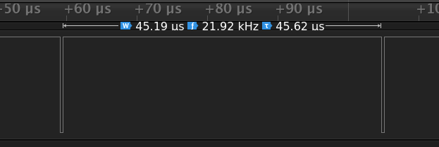
Spoiler alert: it does not
45.19µS! That’s almost half the speed we’d expect with a similarly implemented
loop. Let’s take a look at the disassembly of our ARM loop and see what we can
see (comments added on right):
080000c0 <_Z4loopv>:
 80000c0:       2280            movs    r2, #128        ; Load 0x80
 80000c2:       4b07            ldr     r3, [pc, #28]   ; Load GPIOB memory address
 80000c4:       0052            lsls    r2, r2, #1      ; Logical shift 0x80 left once to get 0x100
 80000c6:       601a            str     r2, [r3, #0]    ; Store 0x100 into GPIOB memory addr (set indicator)
 80000c8:       23ff            movs    r3, #255        ; Load loop variable
 80000ca:       46c0            nop                     ; Loop body
 80000cc:       3b01            subs    r3, #1          ; Subtract one from loop counter
 80000ce:       b2db            uxtb    r3, r3          ; Extend 8 bit value to 32 bit
 80000d0:       2b00            cmp     r3, #0          ; Compare to 0
 80000d2:       d1fa            bne.n   80000ca <_Z4loopv+0xa> ; Jump back into loop if != 0
 80000d4:       2280            movs    r2, #128        ; Load 0x80
 80000d6:       4b02            ldr     r3, [pc, #8]    ; Load GPIOB memory address
 80000d8:       0452            lsls    r2, r2, #17     ; Left shift again to get bit 8 set
 80000da:       601a            str     r2, [r3, #0]    ; Clear GPIOB pin 8
 80000dc:       4770            bx      lr              ; Return
 80000de:       46c0            nop                     ; (Dead code for alignment)
 80000e0:       48000418        stmdami r0, {r3, r4, sl}; GPIOB memory mapped IO location
The core of our loop seems pretty similar to the AVR: we execute a nop,
a subtract, compare and a branch.
We also have a sign-extend instruction on our loop counter in r3, which we
can eliminate by converting our uint8_t loop counter to a
uint32_t.
But there are some goings on
in the lean-in and lead-out that are a bit confusing - such as why are we
loading 0x80 and left shifting it instead of loading 0x100?
The answer is that
our ARM core isn’t actually running the ARM instruction set - it’s running in
Thumb mode.
Thumb mode
One of the downsides of a RISC ISA is that you tend to need more
instructions in your binary than you would on a CISC ISA with more operations
baked into silicon as a single opcode. For embedded and other space-sensitive
applications, having lots of 32-bit ARM instructions can waste precious program
ROM. To get around this, ARM created the Thumb instruction set, with (mostly)
16-bit instructions. So long as you’re mostly using common instructions, this
can easily close to double your instruction density! But like all things, there
are tradeoffs. One visible here is that the movs Thumb instruction only
supports immediate values in the range [0..255], so loading our bit constant
(1 << 8)cannot be done as a single movs - we have to load (1 << 7) and
then shift it once more once it’s loaded to a register. The alternative for
loading constants is what’s been done by GCC for the memory-mapped IO region
for port B, which is to embed it as part of the function below the bx lr
return call - 0x48000418 is our MMIO location, which is loaded using
ldr r3, [pc, #28] to load a full word constant from memory. Presumably our
0x100 constant is not big enough for GCC to think it worth using the
same trick here.
So let’s calculate our our cycle counts for the ARM code as we did for the AVR,
using this
list of instructions.
We have a couple cycles overhead for our lead in and lead out, but the core of
our loop has the following cycle characteristics:
Calculating it out, that’s approximately 7 + (7 * 255) + 6 = 1,789 cycles! Close to double
the count of our AVR code. At 48MHz, that’s a theoretical execution time of
37.27µS. Our actual measured time (45.19µS) is somewhat slower - my
assumption is that this is due to flash wait states, as the STM32F070 this test
was run on has 1 wait state for clock speeds > 24MHz. These delays should only
be incurred for non-linear flash accesses, and so our repeated loop branching
is a worse-case scenario here. Inserting an extra cycle
into our loop for a prefetch miss results in a total cycle count of 2,053, and
an expected runtime of 42.77µS, which is much closer to our measured time.
What should I take away from all this
At the end of digging into all this, I have a newfound respect for the AVR
architecture - single cycle IO access makes it much more competitive for
applications with lots of standalone IO calls (but perhaps not for standard
protocols like SPI, which tend
to be offloaded to baked-in peripherals on the ARM cores, and with DMA support
can be extremely powerful).
It’s also useful to be aware of the limitations and quirks of the Thumb
instruction set - keeping constants small, avoiding spurious resize
instructions and minimizing branches are ways to eke more performance out of
tightly looped controllers. If I were to summarize some key takeaways, they
might be:
A higher clock speed doesn’t necessarily mean more performance
Cycle count estimations can be useful for ballpark runtime calculation
If you need to know for sure, measure it! It’s easy to make mistaken
assumptions, but luckily it can also be simple to verify them.
Thu, Sep 13, 2018Companion code for this post available on Github
In the
previous section,
we covered alternate functions, and configured a log console over UART.
This time, we’ll take a look at the SPI peripherals available on the STM32F0,
use them to quickly shift out data to some shift registers, and then demonstrate
how to then offload that transfer from the main CPU using DMA. Since we have
some other ICs involved here, instead of the simple breakout from before I will
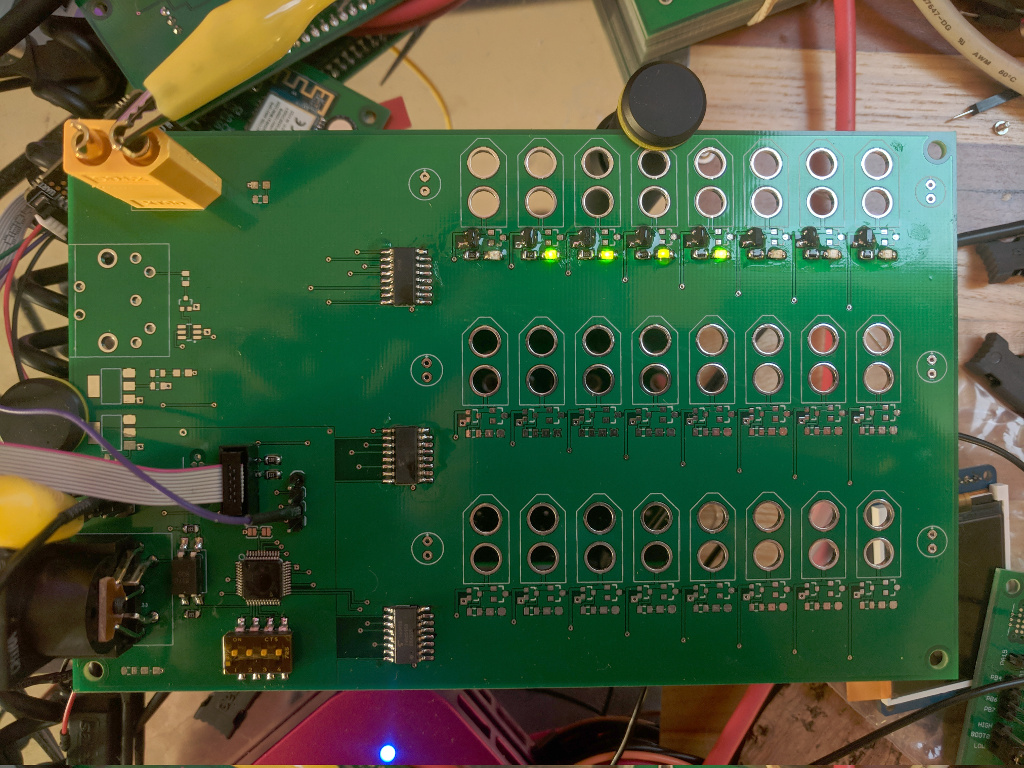
be using this MIDI relay board as a demonstration piece:
MIDI solenoid control board (a work in progress).
The ICs of interest here are the row of shift registers down the middle,
each of which is responsible for driving the eight FETs by each of the solenoid
connection points. For this example I have only populated the first row of 8,
but this will be enough to demonstrate. Our STM32F070 IC, SWD header and uart
breakout are visible in the bottom left corner of the board. Shift registers,
for those that aren’t familiar, allow one to take serial data and convert it to
a parallel output. These ICs are
74HC595
models, which are 8-bit shift registers with separate shift and storage
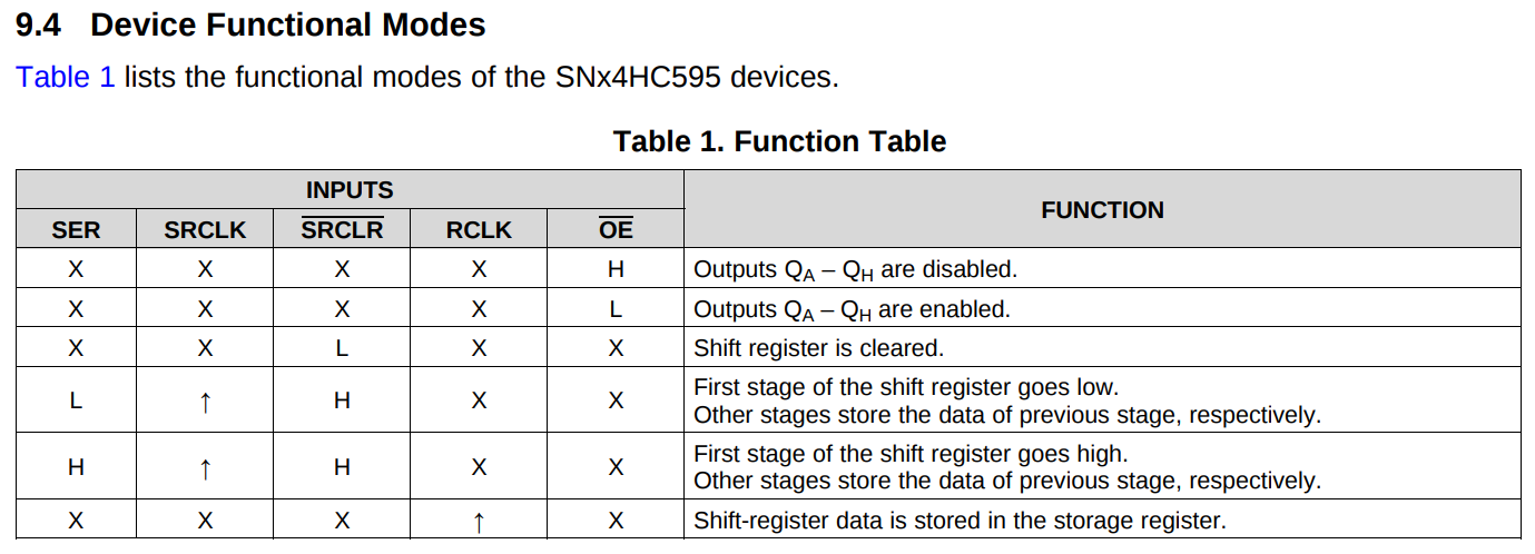
registers. But how do we get the data in there? From the datasheet, we can find
this table defining the behaviour as we manipulate the control inputs:
Functional description of the 595 shift register
So in order to shift data, we cycle SRCLK and on each rising edge the data
on SER will be shifted in to the shift register, and all data presently in
the shift register will be shifted over one. Once we have repeated this to load
as much data as we might want to, we can then clock the RCLK line from low to
high to shift the data in the shift register to the storage register, making it
visible on the outputs.
Now, to drive this we could write a method that carefully takes each byte we
want to send and iterates along each bit inside it, manually toggling the SER
and SRCLK lines to shift data in. But this would be tedious, slow, and
duplicating a built-in peripheral that does exactly the same thing: SPI!
Serial Peripheral Interface
The SPI protocol is a simple communication interface usually consisting of 4
signals:
MOSI (Master Out Slave In)
MISO (Master In Slave Out)
SCK (Serial ClocK)
SS (Slave Select)
Unlike UART, this protocol has a clock signal - as a result, SPI buses can be
operated at far higher speeds since both sides can know precisely when to
latch each bit. Like UART, it is a duplex - the MOSI and MISO lines are each
unidirectional, and can both transmit data during the same clock pulse.
However, SPI also allows for multiple slaves (and, in more complex setups,
multiple masters) on the same MISO and MOSI lines. In order to prevent
slaves from reading / writing data not intended for them, the Slave Select
signal is used to identify which chip is being addressed. Notably, the SS
signal is active low - this means that we can use our SPI MOSI, SCK and SS
lines to map perfectly to the SER, SRCLK and RCLK lines of our shift registers.
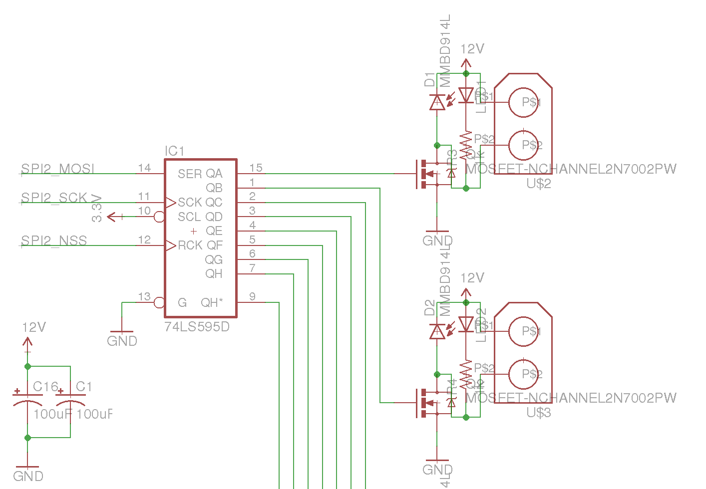
Using this information, we can codify it in our schematic like so:
SPI connections for driving shift register. Additional 595s are fed the same SCK and NSS signals, but chained QH* -> SER.
So now that we have our SPI pins mapped to our shift register (in this case, we
are using PB12-PB15 and the SPI2 peripheral), we can start start work on
initializing our SPI peripheral in preparation for sending data through it.
voidspi_setup() {
// Enable clock for SPI2 peripheral
rcc_periph_clock_enable(RCC_SPI2);
// Configure GPIOB, AF0: SCK = PB13, MISO = PB14, MOSI = PB15
gpio_mode_setup(GPIOB, GPIO_MODE_AF, GPIO_PUPD_NONE, GPIO13 | GPIO14 | GPIO15);
gpio_set_af(GPIOB, GPIO_AF0, GPIO13 | GPIO14 | GPIO15);
// We will be manually controlling the SS pin here, so set it as a normal output
gpio_mode_setup(GPIOB, GPIO_MODE_OUTPUT, GPIO_PUPD_NONE, GPIO12);
// SS is active low, so pull it high for now
gpio_set(GPIOB, GPIO12);
// Reset our peripheral
spi_reset(SPI2);
// Set main SPI settings:
// - The datasheet for the 74HC595 specifies a max frequency at 4.5V of
// 25MHz, but since we're running at 3.3V we'll instead use a 12MHz
// clock, or 1/4 of our main clock speed.
// - Set the clock polarity to be zero at idle
// - Set the clock phase to trigger on the rising edge, as per datasheet
// - Send the most significant bit (MSB) first
spi_init_master(
SPI2,
SPI_CR1_BAUDRATE_FPCLK_DIV_4,
SPI_CR1_CPOL_CLK_TO_0_WHEN_IDLE,
SPI_CR1_CPHA_CLK_TRANSITION_1,
SPI_CR1_MSBFIRST
);
// Since we are manually managing the SS line, we need to move it to
// software control here.
spi_enable_software_slave_management(SPI2);
// We also need to set the value of NSS high, so that our SPI peripheral
// doesn't think it is itself in slave mode.
spi_set_nss_high(SPI2);
// The terminology around directionality can be a little confusing here -
// unidirectional mode means that this is the only chip initiating
// transfers, not that it will ignore any incoming data on the MISO pin.
// Enabling duplex is required to read data back however.
spi_set_unidirectional_mode(SPI2);
// We're using 8 bit, not 16 bit, transfers
spi_set_data_size(SPI2, SPI_CR2_DS_8BIT);
// Enable the peripheral
spi_enable(SPI2);
}
Our SPI peripheral should now be ready to transmit data. In order to make
things easier for us, let’s create a simple helper method that will transmit a
given amount of data over the SPI bus:
voidspi_transfer(uint8_t tx_count, uint8_t *tx_data) {
// Pull CS low to select target. In our case, this just pulls the register
// clock low so that we can lock in the new data at the end of the
// transfer.
gpio_clear(GPIOB, GPIO12);
// For each byte of data we want to transmit
for (uint8_t i =0; i < tx_count; i++) {
// Wait for the peripheral to become ready to transmit (transmit buffer
// empty flag set)
while (!(SPI_SR(SPI2) & SPI_SR_TXE));
// Place the next data in the data register for transmission
SPI_DR8(SPI2) = tx_data[i];
}
// Putting data into the SPI_DR register doesn't block - it will start
// sending the data asynchronously with the main CPU. To make sure that the
// data is finished sending before we pull the register clock high again,
// we wait here until the busy flag is cleared on the SPI peripheral.
while (SPI_SR(SPI2) & SPI_SR_BSY);
// Bring the SS pin high again to latch the new data
gpio_set(GPIOB, GPIO12);
}
So now we should be able to easily clock out data to our shift registers over
SPI. To test this, let’s update our main loop from last time:
intmain() {
// Clock, UART, etc setup
// [...]
// Initialize our SPI peripheral
spi_setup();
// Make a very simple count up display using our 8 LEDs
uint8_t i =0;
while (1) {
i++;
spi_transfer(1, &i);
delay(1000);
}
}
Shift register output
Perfect, we can see that we are slowly counting up. Now, this is obviously a
fairly small application of SPI - we only have 8 bits to transfer here (24 for
a fully populated board); it will take a truly infinitessimal time to push
this data. But if you have a lot of data to move, for example bitmap data you
need to push to a screen, the amount of time it takes to move that data from
memory to the SPI bus might start to become a problem - while you’re looping
over all the data to send and moving it piece by piece to the SPI data
register, you’re losing time to process other events or start drawing the next
frame. Wouldn’t it be great if something so simple as moving data from
memory to a peripheral could be offloaded somehow?
Direct Memory Access
DMA controllers allow us to offload certain types of data shuffling from the
main processor, freeing it to get on with business. In the STM32F0 series, the
controller can be used to move data between two peripherals, from a peripheral
into memory, or from memory to a peripheral. For this example, we’re going to
use it to copy data from memory to our SPI peripheral, so that it can be sent
our to our shift registers. Each DMA controller has multiple channels, and
those channels are all bound to specific peripheral functions.
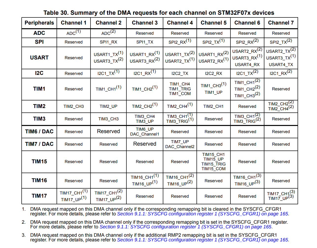
If we take a look at the
STM32F0 series datasheet,
we can find a table showing us which channels map to which peripherals.
DMA channel mapping for the STM32F070 MCU
Based on this, we can see that in order to transmit data on SPI2, we need to
use DMA channel 5. So let’s start configuring our DMA controller:
voiddma_init() {
// Enable DMA clock
rcc_periph_clock_enable(RCC_DMA1);
// In order to use SPI2_TX, we need DMA 1 Channel 5
dma_channel_reset(DMA1, DMA_CHANNEL5);
// SPI2 data register as output
dma_set_peripheral_address(DMA1, DMA_CHANNEL5, (uint32_t)&SPI2_DR);
// We will be using system memory as the source data
dma_set_read_from_memory(DMA1, DMA_CHANNEL5);
// Memory increment mode needs to be turned on, so that if we're sending
// multiple bytes the DMA controller actually sends a series of bytes,
// instead of the same byte multiple times.
dma_enable_memory_increment_mode(DMA1, DMA_CHANNEL5);
// Contrarily, the peripheral does not need to be incremented - the SPI
// data register doesn't move around as we write to it.
dma_disable_peripheral_increment_mode(DMA1, DMA_CHANNEL5);
// We want to use 8 bit transfers
dma_set_peripheral_size(DMA1, DMA_CHANNEL5, DMA_CCR_PSIZE_8BIT);
dma_set_memory_size(DMA1, DMA_CHANNEL5, DMA_CCR_MSIZE_8BIT);
// We don't have any other DMA transfers going, but if we did we can use
// priorities to try to ensure time-critical transfers are not interrupted
// by others. In this case, it is alone.
dma_set_priority(DMA1, DMA_CHANNEL5, DMA_CCR_PL_LOW);
// Since we need to pull the register clock high after the transfer is
// complete, enable transfer complete interrupts.
dma_enable_transfer_complete_interrupt(DMA1, DMA_CHANNEL5);
// We also need to enable the relevant interrupt in the interrupt
// controller, and assign it a priority.
nvic_set_priority(NVIC_DMA1_CHANNEL4_5_IRQ, 0);
nvic_enable_irq(NVIC_DMA1_CHANNEL4_5_IRQ);
}
So now, our DMA controller is all set up to push data from memory to SPI2’s
transmit buffer. But note that in our setup we didn’t specify our source memory
location or how much data we’re sending - let’s add a method for that now
voiddma_start(void*data, size_t data_size) {
// Note - manipulating the memory address/size of the DMA controller cannot
// be done while the channel is enabled. Ensure any previous transfer has
// completed and the channel is disabled before you start another transfer.
// Tell the DMA controller to start reading memory data from this address
dma_set_memory_address(DMA1, DMA_CHANNEL5, (uint32_t)data);
// Configure the number of bytes to transfer
dma_set_number_of_data(DMA1, DMA_CHANNEL5, data_size);
// Enable the DMA channel.
dma_enable_channel(DMA1, DMA_CHANNEL5);
// Since we're manually controlling our register clock, move it low now
gpio_clear(GPIOB, GPIO12);
// Finally, enable SPI DMA transmit. This call is what actually starts the
// DMA transfer.
spi_enable_tx_dma(SPI2);
}
But this is only half the process - we also need to handle the termination
condition of the DMA transfer, so that we can move our register clock high
again to latch the data. So for this, we need to implement an interrupt handler
for our DMA channel. DMA channels 4 and 5 use the same ISR -
dma1_channel4_5_isr - so let’s
implement that now.
voiddma1_channel4_5_isr() {
// Check that we got triggered because the transfer is complete, by
// checking the Transfer Complete Interrupt Flag
if (dma_get_interrupt_flag(DMA1, DMA_CHANNEL5, DMA_TCIF)) {
// If that is why we're here, clear the flag for next time
dma_clear_interrupt_flags(DMA1, DMA_CHANNEL5, DMA_TCIF);
// Like the non-dma version, we don't want to latch the register clock
// until the transfer is actually complete, so wait til the busy flag
// is clear
while (SPI_SR(SPI2) & SPI_SR_BSY);
// Turn our DMA channel back off, in preparation of the next transfer
spi_disable_tx_dma(SPI2);
dma_disable_channel(DMA1, DMA_CHANNEL5);
// Bring the register clock high to latch the transferred data
gpio_set(GPIOB, GPIO12);
}
}
To tie it all together and demonstrate that the DMA transfer is separate from
normal CPU operations, let’s start a DMA transfer and then immediately write
some text over the USART.
intmain() {
// Setup clock, serial, spi, etc
// [...]
// Initialize the DMA controller
dma_init();
// Allocate a nice big slab of data
uint8_t data[1024];
for (int i =0; i <1024; i++) {
data[i] = i;
}
// Begin a DMA transfer using that data
dma_start(data, 1024);
// Immediately start printing some text to our console
printf("Concurrent DMA and USART!\n");
while (true) {
// Nothing
}
return0;
}
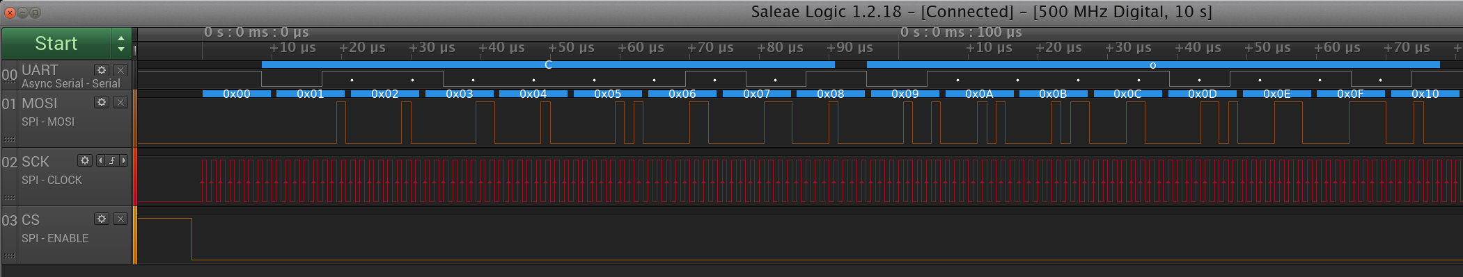
If we now tap the UART and SPI lines on the board with a logic analyzer, we can
observe that we are indeed sending both SPI and UART data concurrently:
Trace of our SPI bus and UART TX
Success! We can see that while the main thread of execution has moved on to
sending data over the USART, the DMA controller has begun sending out kilobyte
of data in the background.
While DMA is still limited by sharing the same memory and peripheral
bus as the processor, and so both must still negotiate if there are bus
conflicts, it is a powerful tool for offloading simpler peripheral operations
in this way. You can even do more complex DMA operations, such as pushing
double-buffering video data bv taking advantage of circular DMA and
the “transfer half complete” interrupt.
As per usual, the code for this post is available on
Github.
The next post in this series, on CANBus, can be found
here
Wed, Sep 12, 2018Companion code for this post available on Github
In the
previous section,
we covered the basics of compiling for, and uploading to, an STM32F0 series MCU
using
libopencm3 to make an LED blink.
This time, we’ll take a look at alternate pin functions, and use one of the
four USARTs on our chip to send information back to our host machine. As
before, this is all based on a small breakout board for the
STM32F070CBT6, but can be applied to
other boards and MCUs.
Alternate functions
In addition to acting as General Purpose I/Os, many of the pins on the STM32
microcontrollers have one or more alternate functions. These alternate
functions are tied to subsystems inside the MCU, such as one or more SPI, I2C,
USART, Timer, DMA or other peripherals.
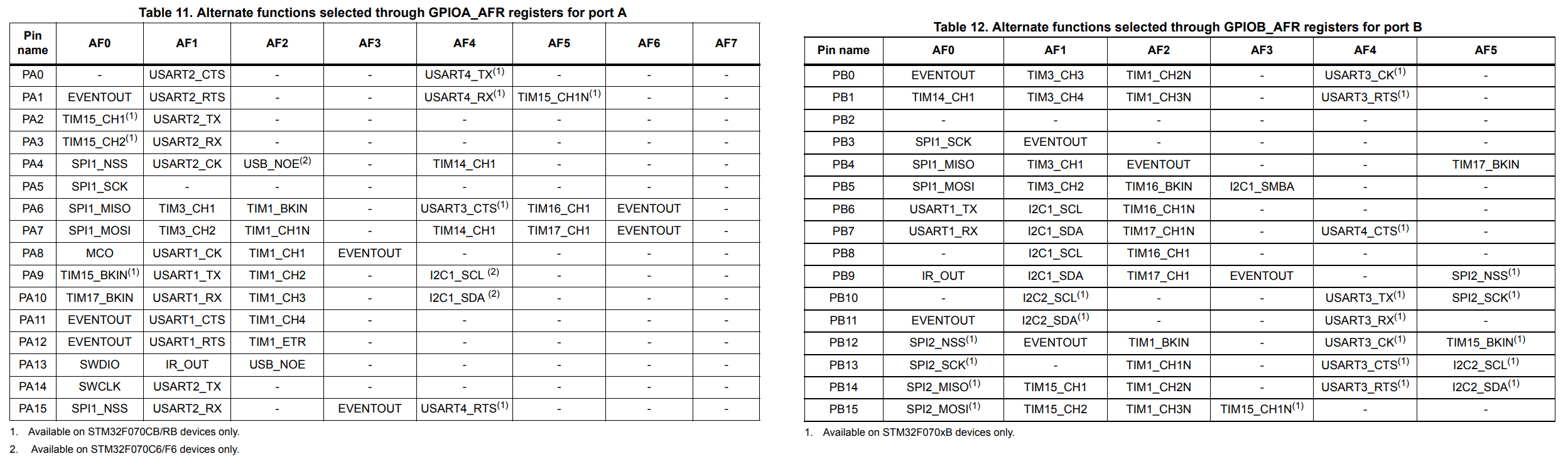
If we take a look at the
datasheet
for the STM32F070, we see that there are up to 8 possible alternate functions
per pin on ports A and B.
Alternate function tables for STM32F070
Note that some peripherals are accessible on multiple different sets of pins as
alternate functions - this can help with routing your designs later, since you
can to some degree shuffle your pins around to move them closer to the other
components to which they connect. An example would be SPI1, which can be
accessed either as alternate function 0 on port A pins 5-7, or as alternate
function 0 on port B, pins 3-5. But for this example, we will be looking at
USART1, which from the tables above we can see is AF1 on PA9 (TX) and PA10
(RX).
To quickly recap -
USARTs allow for sending relatively low-speed data using a simple 1-wire per
direction protocol. Each line is kept high, until a transmission begins and the
sender pulls the line low for a predefined time to signal a start condition
(start bit). The sender then, using it’s own clock, pulls the line low for
logic 1 and high for logic 0 to transmit a configurable number of bits to the
receiver, followed by an optional parity bit and stop bit. The receiver
calculates the time elapsed after the start condition using it’s own clock, and
recovers the data. While simple to implement, they have a drawback in that they
lack a separate clock line, and must rely on both sides keeping close enough time to
understand each other. For our case, they work great for sending back debug
information to our host computer. So let’s update our example from last time,
to include a section that initializes USART1 with a baudrate of 115200, and the
transmit pin connected to Port A Pin 9.
staticvoidusart_setup() {
// For the peripheral to work, we need to enable it's clock
rcc_periph_clock_enable(RCC_USART1);
// From the datasheet for the STM32F0 series of chips (Page 30, Table 11)
// we know that the USART1 peripheral has it's TX line connected as
// alternate function 1 on port A pin 9.
// In order to use this pin for the alternate function, we need to set the
// mode to GPIO_MODE_AF (alternate function). We also do not need a pullup
// or pulldown resistor on this pin, since the peripheral will handle
// keeping the line high when nothing is being transmitted.
gpio_mode_setup(GPIOA, GPIO_MODE_AF, GPIO_PUPD_NONE, GPIO9);
// Now that we have put the pin into alternate function mode, we need to
// select which alternate function to use. PA9 can be used for several
// alternate functions - Timer 15, USART1 TX, Timer 1, and on some devices
// I2C. Here, we want alternate function 1 (USART1_TX)
gpio_set_af(GPIOA, GPIO_AF1, GPIO9);
// Now that the pins are configured, we can configure the USART itself.
// First, let's set the baud rate at 115200
usart_set_baudrate(USART1, 115200);
// Each datum is 8 bits
usart_set_databits(USART1, 8);
// No parity bit
usart_set_parity(USART1, USART_PARITY_NONE);
// One stop bit
usart_set_stopbits(USART1, USART_CR2_STOPBITS_1);
// For a debug console, we only need unidirectional transmit
usart_set_mode(USART1, USART_MODE_TX);
// No flow control
usart_set_flow_control(USART1, USART_FLOWCONTROL_NONE);
// Enable the peripheral
usart_enable(USART1);
// Optional extra - disable buffering on stdout.
// Buffering doesn't save us any syscall overhead on embedded, and
// can be the source of what seem like bugs.
setbuf(stdout, NULL);
}
Now that we have this, we can write some helper functions for logging strings
to the serial console:
Once again, run make flash to compile and upload to your target. Now, take
the ground and VCC lines of the serial interface on the bottom of your Black
Magic probe, and connect them to the ground / positive rails of your test
board. Then connect the RX line on the probe (purple wire) to the TX pin on
your board. You can then start displaying the serial output by running
$ screen /dev/ttyACM1 115200
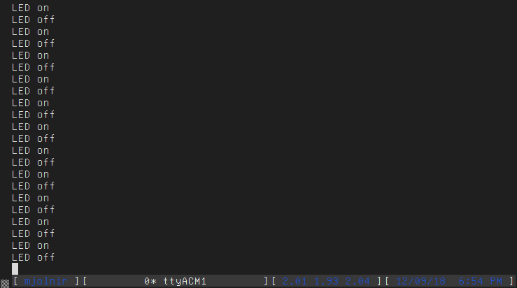
After a couple seconds, you should have a similarly riveting console output:
Basic serial console logs, using screen
This is ok, but what if we want to actually format data into our console logs?
If we have size constraints we may roll our own integer/floating point
serialization logic, but printf already exists and provides a nice interface
- so why not take printf and allow it to write to the serial console?
Replacing POSIX calls
When targeting embedded systems, one tends to compile without linking against
a full standard library - since there is no operating system, syscalls such as
open, read and exit don’t really make sense. This is part of what is done
by linking with -lnosys - we replace these syscalls with stub functions, that
do nothing. For example, the POSIX write call eventually calls through to a
function with the prototype:
(I believe that this list of prototypes covers the syscalls that can be implemented in this manner).
So, if printf will eventually call write, if we re-implement the backing
_write method to instead push that data to the serial console, we can
effectively redirect stdout and stderr somewhere we can see them - we could
even redirect stdout to one USART and stderr to another! But for
simplicity, let’s just pipe both to USART1 which we set up earlier:
// Don't forget to allow external linkage if this is C++ code
extern"C" {
ssize_t _write(int file, constchar*ptr, ssize_t len);
}
int _write(int file, constchar*ptr, ssize_t len) {
// If the target file isn't stdout/stderr, then return an error
// since we don't _actually_ support file handles
if (file != STDOUT_FILENO && file != STDERR_FILENO) {
// Set the errno code (requires errno.h)
errno = EIO;
return-1;
}
// Keep i defined outside the loop so we can return it
int i;
for (i =0; i < len; i++) {
// If we get a newline character, also be sure to send the carriage
// return character first, otherwise the serial console may not
// actually return to the left.
if (ptr[i] =='\n') {
usart_send_blocking(USART1, '\r');
}
// Write the character to send to the USART1 transmit buffer, and block
// until it has been sent.
usart_send_blocking(USART1, ptr[i]);
}
// Return the number of bytes we sent
return i;
}
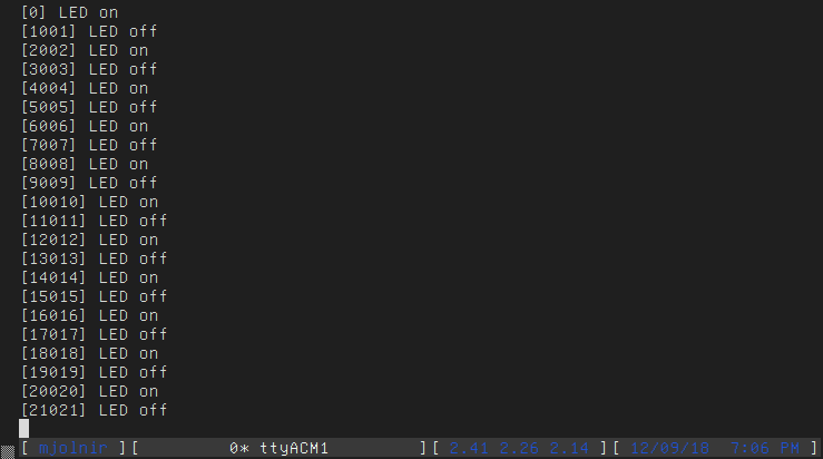
Now, we could jazz up that print output from before by prefixing all of our log
messages with the current monotonic time:
intmain() {
// Previously defined clock, USART, etc... setup elided
// [...]
while (true) {
printf("[%lld] LED on\n", millis());
gpio_set(GPIOA, GPIO11);
delay(1000);
printf("[%lld] LED off\n", millis());
gpio_clear(GPIOA, GPIO11);
delay(1000);
}
}
Serial console logs, with formatting
As before, the final source code for this post is available
on Github.
In the
next post,
we will go over SPI and memory-to-peripheral DMA.
Tue, Sep 11, 2018Companion code for this post available on Github
For many years now, I have found myself building (admittedly small) electronics
projects, and for almost all of that time I have found myself reaching for the
same microcontroller: the humble Atmega 328p that powers so many Arduinos (and
Arduino clones!). This choice was driven by the fact that being an
Arduino-compatible MCU meant I could take advantage of the huge library of
code built for the Arduino platform. However, the choice is somewhat limiting -
with only 16KiB of flash and 2KiB of sram, some applications were simply
infeasible within that range. In addition, the relatively slow 16MHz top speed
can make high-data-rate applications, like display driving, somewhat of a
challenge.
Luckily, there are a number of increasingly cheap ARM based MCUs on the market.
In particular, ST has an excellent lineup, including a ‘value line’ of F0
series MCUs that offer a lot of features (128K flash, 16K sram, multiple SPI /
I2C / Timer / DMA peripherals) for relatively cheap. However, a lot of the
proprietary development environments (such as the graphical STMCube software)
seem to me overly complex, and make it difficult to use preferred editors /
development toolchains. Luckily, there is an open source low-level hardware
abstraction library with coverage for the STM32 series of MCUs, called
libopencm3.
Using this, it is easy to write portable C(++) code that can easily be deployed
using only GNU tools. In this tutorial, I will attempt to cover the basics of
starting a new project with libopencm3, compiling, uploading code, and the
use of the SysTick peripheral.
The full source code for this tutorial, along with the EAGLE and Gerber files
for the breakout board I used, are available in this
Github repo.
Equipment
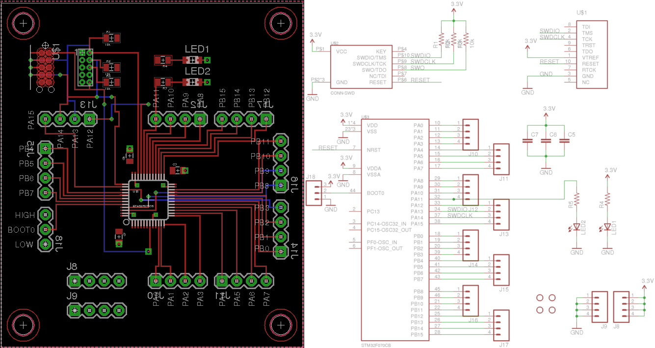
Since my goal was to be able to use these MCUs in my own designs, I am not
using an off-the-shelf development board from ST, but an extremely basic
breakout of my own design with nothing but an
STM32F070CBT6, a Single-Wire Debug
(SWD) header and all IO pins on the MCU broken out to .1” headers. These
instructions should however work for any board with an STM32FX part, so long as
it has a SWD header.
Breakout board and schematic. Source materials available in Github.
The only other important piece of kit is a
Black Magic probe.
The BMP is a fantastic little device - it provides a GDB server that makes it
simple to upload code to the MCU, debug it, and also has a UART interface so
that you can wire it up to get a debug console. It can be found online for
~$60USD at time of writing.
Foundation
The very first thing we are going to do is acquire a copy of libopencm3 to
compile against. In order to make sure that we don’t end up with any dependency
drift, I am going to add it as a
submodule
to our new git project. So let’s
start by creating a new project, and cloning it in:
Now, we need to build opencm3 so that we can link against it later.
If you do not have GCC for ARM installed, you may need to install it now.
For Debian and kin, the following will install everything you might need for
this tutorial:
Now, we can drop into the libopencm3 dir and build.
Note that if you have custom CFLAGS or CXXFLAGS set for your host machine,
you may need to unset them if they are unsupported by gcc-arm.
$ pushd libopencm3
$ unset CFLAGS && unset CXXFLAGS # You may not need to do this
$ make
$ popd
Now that we have our library ready, it’s time to start writing some code. To
begin, let’s just start by blinking the LED I have attached to pin PA11. If you
are using a different test board, you may need to sub out GPIOA and GPIO11
to match the port and pin you are using instead.
#include<libopencm3/stm32/rcc.h>#include<libopencm3/stm32/gpio.h>intmain() {
// First, let's ensure that our clock is running off the high-speed
// internal oscillator (HSI) at 48MHz
rcc_clock_setup_in_hsi_out_48mhz();
// Since our LED is on GPIO bank A, we need to enable
// the peripheral clock to this GPIO bank in order to use it.
rcc_periph_clock_enable(RCC_GPIOA);
// Our test LED is connected to Port A pin 11, so let's set it as output
gpio_mode_setup(GPIOA, GPIO_MODE_OUTPUT, GPIO_PUPD_NONE, GPIO11);
// Now, let's forever toggle this LED back and forth
while (true) {
gpio_toggle(GPIOA, GPIO11);
}
return0;
}
This is very basic, but it’s something we can compile to ensure we’re able to
load code at all. Later on we will refine this example. But first, we need to
build a linker script
Linker scripts
As part of compiling our code, we need to specify where in our MCU memory
to place both the code as well as our memory. In order to do this, we first
need to look up the address space map for our CPU. From the STM32F070
datasheet, we see that the ‘Flash Memory’ block resides at 0x08000000 and is
128KiB in size, while the main ram (SRAM) lives at 0x20000000 and is 16KiB in
size. Armed with this information, we can create our linker script with these
two sections:
OpenCM3 proves the cortex-m-generic.ld script, which takes our rom/ram
definitions to locate the stack, as well as specify the locations of the
.text, .data, .bss and other sections. It’s fairly short, so it’s worth
taking a look if you’re curious about the details of how sections are laid out
in memory.
Building
Now that we have our device-specific linker data, we can get to compiling. I’ve
posted this example project
on Github
including the
full Makefile
that defines the build rules necessary to compile our project. The core
variables in that makefile are
OBJS: The list of .o files to compile. Since we only have the one source
file, main.cpp, we have only one object file, main.o.
OPENCM3_DIR: The location of opencm3 relative to our project. In this case,
it is in the same directory.
LDSCRIPT: The linker script to use. Set this to the one we made earlier.
LIBNAME and DEPS: The precise chip variant that we are compiling for.
This controls which includes are matched from opencm3, and which support
library is linked against.
To try and keep this short, I won’t go over the entire makefile here. However,
here are the two commands, in full, used to compile and link our simple binary.
I have gone through and annotated each flag, which will hopefully explain why
they are present.
$ arm-none-eabi-g++ \
    -Os \ # Optimize for code size
    -ggdb3 \ # Include additional debug info
    -mthumb \ # Use thumb mode (smaller instructions)
    -mcpu=cortex-m0 \ # Target CPU is a Cortex M0 series
    -msoft-float \ # Software floating-point calculations
    -Wall \ # Enable most compiler warnings
    -Wextra \ # Enable extra compiler warnings
    -Wundef \ # Warn about non-macros in #if statements
    -Wshadow \ # Enable warnings when variables are shadowed
    -Wredundant-decls \ # Warn if anything is declared more than once
    -Weffc++ \ # Warn about structures that violate effective C++ guidelines
    -fno-common \ # Do not pool globals, generates error if global redefined
    -ffunction-sections \ # Generate separate ELF section for each function
    -fdata-sections \ # Enable elf section per variable
    -std=c++11 \ # Use C++11 standard
    -MD \ # Write .d files with dependency data
    -DSTM32F0 \ # Define the series of MCU we are using. This controls the
              \ # include pathways inside libopencm3.
    -I./libopencm3/include \ # Include the opencm3 header files
    -o main.o \ # Output filename
    -c main.cpp # Input file to compile

$ arm-none-eabi-gcc \
    --static \ # Don't try and use shared libraries
    -nostartfiles \ # No standard lib startup files
    -Tstm32f0.ld \ # Use the linker script we defined earlier
    -mthumb \ # Thumb instruction set for smaller code
    -mcpu=cortex-m0 \ # Cortex M0 series MCU
    -msoft-float \ # Software floating point
    -ggdb3 \ # Include detailed debug info
    -Wl,-Map=main.map \ # Generate a memory map in 'main.map'
    -Wl,--cref \ # Output a cross-reference table to the mem map
    -Wl,--gc-sections \ # Perform dead-code elimination
    -L./libopencm3/lib \ # Link against opencm3 libraries
    main.o \ # Our input object(s)
    -lopencm3_stm32f0 \ # The opencm3 library for our chip
    \ # Begin and end group here allow resolving of circular dependencies
    \ # while linking. This links against some common libs:
    \ # -lc: the standard C library
    \ # -lgcc: GCC-provided subroutines
    \ # -lnosys: Stub library with empty definitions for POSIX functions
    -Wl,--start-group -lc -lgcc -lnosys -Wl,--end-group
    -o main.elf # Our output binary
Once I’ve built my code, I also like to print a quick summary of the size so
that I can track how much of my flash and memory is currently consumed. For
this, we can use the arm-none-eabi version of size:
$ arm-none-eabi-size main.elf
  text    data     bss     dec     hex filename
  7832    2120      60   10020    2724 main.elf
So far we’re already using 7k of flash data, and 2k of initialized memory. Only
60 bytes of globally allocated variables however! Now that we have our binary,
it’s time to flash it to our microcontroller.
Flashing
In order to load this code, we’re going to turn to GDB. Since our Black Magic
Probe runs a GDB server, we use it as a remote target. First, ensure that the
10-pin SWD cable is connected to your board in the correct orientation. You
must also be sure to supply power to your board - the BMP will not supply power
to the board itself. Once you’ve done this, we can open up arm-none-eabi-gdb:
$ arm-none-eabi-gdb main.elf
# First, we need to tell GDB to use our BMP as a remote target.
# /dev/ttyACM0 is where it shows up on my machine, but YMMV
(gdb) target extended-remote /dev/ttyACM0
# Now that we are connected, we need to scan for devices to attach to over
# Single Wire Debug
(gdb) monitor swdp_scan
Target voltage: 3.3V
Available Targets:
No. Att Driver
1 STM32F07
# Perfect - our chip is powered and recognizable to GDB.
# Now we can attach to it
(gdb) attach 1# Now that we're connected, we can upload our code
(gdb) load
Loading section .text, size 0x1d5c lma 0x8000000
Loading section .ARM.extab, size 0x30 lma 0x8001d5c
Loading section .ARM.exidx, size 0xd0 lma 0x8001d8c
Loading section .data, size 0x848 lma 0x8001e5c
Start address 0x800033c, load size 9892
Transfer rate: 13 KB/sec, 760 bytes/write.
# We can now run the program as though it were a local binary
(gdb) run
The program being debugged has been started already.
Start it from the beginning? (y or n) y
Starting program: main.elf
This series of steps has been formalized in the gdb script bmp_flash.scr in
the Github repo
for this tutorial, and can be invoked using the flash make target.
You should see that the LED has appeared to turn on solidly. Unfortunately, at
48MHz, it’s a little hard for the human eye to notice it pulsing. Let’s make it
a little more obvious by pulsing it on and off each second, and to do so we’ll
use our first proper peripheral: the SysTick timer.
SysTick
The SysTick timer on the STM32 series of MCUs is a simple countdown timer,
which triggers an interrupt every time the counter reaches zero, then reloads
the counter value from a specified reload register. Since we know that our CPU
frequency is 48MHz, if we want to get an approximately real time clock pulse
every millisecond, we can configure our systick timer to reload with a value of
48000000 / 1000 = 48000. Then, every time the interrupt fires, we can increment
a ‘milliseconds’ counter that we can then check against to implement a delay
operation.
// I'll be using fixed-size types
#include<stdint.h>// Include the systick header
#include<libopencm3/cm3/systick.h>// Important note for C++: in order for interrupt routines to work, they MUST
// have the exact name expected by the interrupt framework. However, C++ will
// by default mangle names (to allow for function overloading, etc) and so if
// left to it's own devices will cause your ISR to never be called. To force it
// to use the correct name, we must declare the function inside an 'extern C'
// block, as below.
// For more details, see https://en.cppreference.com/w/cpp/language/language_linkage
extern"C" {
void sys_tick_handler(void);
}
// Storage for our monotonic system clock.
// Note that it needs to be volatile since we're modifying it from an interrupt.
staticvolatile uint64_t _millis =0;
staticvoidsystick_setup() {
// Set the systick clock source to our main clock
systick_set_clocksource(STK_CSR_CLKSOURCE_AHB);
// Clear the Current Value Register so that we start at 0
STK_CVR =0;
// In order to trigger an interrupt every millisecond, we can set the reload
// value to be the speed of the processor / 1000 - 1
systick_set_reload(rcc_ahb_frequency /1000-1);
// Enable interrupts from the system tick clock
systick_interrupt_enable();
// Enable the system tick counter
systick_counter_enable();
}
// Get the current value of the millis counter
uint64_t millis() {
return _millis;
}
// This is our interrupt handler for the systick reload interrupt.
// The full list of interrupt services routines that can be implemented is
// listed in libopencm3/include/libopencm3/stm32/f0/nvic.h
voidsys_tick_handler(void) {
// Increment our monotonic clock
_millis++;
}
// Delay a given number of milliseconds in a blocking manner
voiddelay(uint64_t duration) {
const uint64_t until = millis() + duration;
while (millis() < until);
}
Once we have this framework, we can update our main from before to make
our blinking more obvious.
intmain() {
// Previously defined clock and GPIO setup elided
// [...]
// Initialize our systick timer
systick_setup();
while (true) {
gpio_set(GPIOA, GPIO11);
delay(1000);
gpio_clear(GPIOA, GPIO11);
delay(1000);
}
}
Once we’ve made these changes, we can now make flash to compile and upload
our program. We should now see our LED blink at a nice visible rate.
Expected result: a 0.5Hz blink.
In the
next post, we take a look at
alternate functions, USART, and redirecting printf to serial console.
I have an ever-increasing number of small projects and deployments that I
use either internally or with some availability to the public, and
have been relying on Kubernetes to make managing them
easy. Not too long ago, I started adding a liveness probe to each pod
definition as a contingency against a hung runtime. My pod definition at the
time looked like this example from my
Aflame
project:
This worked fine, and I was able to verify that nodes that failed the ping test
would be taken down. However, some weeks later I was poking around and realized
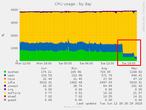
that CPU utilization on my server was significantly higher than I would expect.
Note the recent spike in CPU utilization
Looking at htop, it was difficult to see a precise culprit, except for
a large number of processes called erl_child_setup coming into
existence, pegging a CPU core and disappearing again. After googling around, I
landed on the
source code
for this task and found this section of main:
/* We close all fds except the uds from beam.
All other fds from now on will have the
CLOEXEC flags set on them. This means that we
only have to close a very limited number of fds
after we fork before the exec. */#if defined(HAVE_CLOSEFROM)
closefrom(4);
#else
for (i =4; i < max_files; i++)
#if defined(__ANDROID__)
if (i != system_properties_fd())
#endif
(void) close(i);
#endif
According to the ps output on my system, max_files was getting set to
1,048,576 - so every time this program run, it was hot looping over a million
possible file descriptors and calling close on each! No wonder it was
resulting in so much system time. But what was actually causing all of these
erl_child_setup calls? I had initially suspected a misbehaving deployment
code, but the spike in load lined up with when I added the liveness checks. It
turns out that the relxping command is surprisingly heavyweight; or at
least ends up that way when run in an environment with a very high max file
count, which was the case under docker.
The fix
In order to fix this, I altered my liveness probe to run the ping check with a
low ulimit on the number of open files. We still need to loop, but we are at
least looping over a considerably more restrained number of descriptors.
I also took the
opportunity to increase the interval between checks, since the default check
period is rather quick.
Note that in order to get softlimit in your container, you may need to
rebuild with daemontools package installed, or another source that contains
a limit utility.
Noticably reduced CPU usage
With these changes, system load rapidly dropped from nearly 20 to a more
reasonable 3. The default performance of this wrapper would likely be helped by
an adoption of the closefrom syscall into the Linux kernel, but unfortunately
the only references I can find to this are
a pessimistic ticket from 2009
and an unmerged
patch from Zheng Liu in 2014.
Mon, Mar 26, 2018Companion code for this post available on Github
Recently, I did a
small writeup
on creating natively implemented functions (NIFs) in Erlang. But as was brought
up by several people on reddit and lobste.rs, that example did not account for
any sort of coöperative scheduling with the VM.
The BEAM has one scheduler per CPU core, and these (and, in later versions of
Erlang, the dirty schedulers) are the executors on which all code is run.
In order for the BEAm to try and guarantee a soft-real-time execution
environment, it needs to be able to track how much work each process has done,
so that it can keep CPU hogs in check and not starve other processes.
To do this, it uses the concept of reductions. Each time a statement is
evaluated (reduced), the number of reductions performed by that process is
incremented, until it reaches a set limit and the process is context switched
out.
If we take a look at the erl_nif man page, we can see that there is one method
that deals with accounting for nif time: enif_consume_timeslice. This method
expects to be called relatively regularly from your NIF, with an argument that
is the percentage of a time slice that you believe you have used since the last
time you called that method. The idea of a time slice is somewhat lackluster in
its specificity:
The time is specified as a percent of the timeslice that a process is allowed
to execute Erlang code until it can be suspended to give time for other
runnable processes. The scheduling timeslice is not an exact entity, but can
usually be approximated to about 1 millisecond.
If we take a look at the actual
implementation
we can see what’s actually happening here:
When we call this method, we increase the number of reductions this process has
executed by CONTEXT_REDS (the number of reductions a process may perform
before it should be context-switched out) divided by our percentage.
So far so good. But now, we need to see how we can actually restructure our
code to allow it to be context switched out.
The best way to do this is to use the
primitive enif_schedule_nif, which allows you to specify a function pointer
and arguments that should be called to continue your calculations. Note that
the NIF scheduled in this way does not need to be exported - meaning that it is
fairly safe to create helper NIFs under the assumption that end users will not
try and call them. So let’s take a look at how we might re-write our
Levenshtein example to allow it to perform work in chunks:
// The first thing you'll want to do is create a struct to maintain any
// internal state you want to pass between calls to your NIF.
// In this case, I need to keep track of my matrix, the input strings,
// and which x, y position I had iterated up to.
struct LevenshteinState {
// The matrix being used to calculate the distance
unsignedint*matrix;
// The input strings + their sizes
unsignedchar*s1;
unsigned s1len;
unsignedchar*s2;
unsigned s2len;
// The index of the last processed row of the matrix,
// so that the next iteration can pick up where we left off
unsignedint lastX;
unsignedint lastY;
};
// Now, let's rewrite our entry point so that all it does is read in the
// command arguments, validate them and then yield a call to our internal NIF
// that will do all the actual work.
static ERL_NIF_TERM erl_levenshtein(ErlNifEnv* env, int argc, const
ERL_NIF_TERM argv[]) {
// Not pictured: verifying argc, the type of the arguments,
// and casting the binaries to ErlNifBinary structs.
// Retrieve the state resource descriptor from our priv data,
// and allocate a new structure
// PrivData here is a custom struct, initialized during our module load
// callback. See the code on github for the full implementation with
// regards to this.
struct PrivData *priv_data = enif_priv_data(env);
struct LevenshteinState* state = enif_alloc_resource(
priv_data->levenshtein_state_resource,
sizeof(struct LevenshteinState)
);
//// Initialize the calculation state
// Allocate our matrix
size_t matrix_size = (
sizeof(unsignedint) * (binary1.size +1) * (binary2.size +1)
);
state->matrix = malloc(matrix_size);
// Copy the binary term info
state->s1 = binary1.data;
state->s1len = binary1.size;
state->s2 = binary2.data;
state->s2len = binary2.size;
// Set our initial X and Y values
state->lastX =1;
state->lastY =1;
// In the full version, here is where I also initialize the first row and
// column of the matrix, in order to simplify the code in the helper NIF.
// Now that the setup is complete, we can call erl_schedule_nif to
// tell the beam our continuation function.
// First, we need to wrap our data resource so that it can be passed
// through the BEAM. enif_make_resource takes our state pointer and returns
// an ERL_NIF_TERM.
ERL_NIF_TERM state_term = enif_make_resource(env, state);
// The NIF name here does not seem to be used for determining what code to
// call, and is likely only used when debugging what code is running.
return enif_schedule_nif(
env,
"levenshtein_yielding", // NIF to call
0, // Flags
erl_levenshtein_yielding,
1,
args
);
Now that the glue code is out of the way, we can create our
erl_levenshtein_yielding method, which for workloads greater than a
millisecond we can expect will be called multiple times for the given input.
It will take a single argument, our wrapped state from before, unwrap it, and
continue wherever the previous call left off.
static ERL_NIF_TERM erl_levenshtein_yielding(ErlNifEnv* env, int argc,
const ERL_NIF_TERM argv[]) {
// Not pictured: argc check
// Extract the state term. In the same way we wrapped it before, we need
// to now unwrap the resource we used to pass our struct through.
struct PrivData *priv_data = enif_priv_data(env);
struct LevenshteinState* state;
if (!enif_get_resource(env, argv[0],
priv_data->levenshtein_state_resource,
((void*) (&state)))) {
return mk_error(env, "bad_internal_state");
}
// Start processing wherever the previous slice left off
constunsignedint xsize = state->s1len +1;
unsignedint x = state->lastX;
unsignedint y = state->lastY;
// Specs for tracking function runtime
struct timespec start_time;
struct timespec current_time;
// Grab the function start time
clock_gettime(CLOCK_MONOTONIC, &start_time);
// Create a tracker for the number of loop iterations we've done.
// This operation count will act as a punctuator for us to check
// whether it's time for us to yield again.
unsignedlong operations =0;
// This is a bit slimy, but is the simplest way to preload
// the x and y loop vars for the first inner loop iteration
goto loop_inner;
// Loop over the matrix
for (x = state->lastX; x <= state->s2len; x++) {
for (y =1; y <= state->s1len; y++) {
loop_inner:
// Ordinary Levenshtein implementation
MATRIX_ELEMENT(state->matrix, xsize, x, y) = MIN3(
MATRIX_ELEMENT(state->matrix, xsize, x-1, y) +1,
MATRIX_ELEMENT(state->matrix, xsize, x, y-1) +1,
MATRIX_ELEMENT(state->matrix, xsize, x-1, y-1) +
(state->s1[y-1] == state->s2[x-1] ?0:1)
);
// For each cell, increment the op count until we hit our
// check threshold.
if (unlikely(operations++> OPERATIONS_BETWEN_TIMECHEKS)) {
// When we do, get the current time
clock_gettime(CLOCK_MONOTONIC, ¤t_time);
// Figure out how many nanoseconds have passed since we started
// calculating
unsignedlong nanoseconds_diff = (
(current_time.tv_nsec - start_time.tv_nsec) +
(current_time.tv_sec - start_time.tv_sec) *1000000000
);
// Convert that to a percentage of a timeslice, assuming that
// a time slice is 1 millisecond.
int slice_percent = (nanoseconds_diff *100) / TIMESLICE_NANOSECONDS;
// enif_consume_timeslice requires a percentage in the range
// 1 <= timeslice <= 100
if (slice_percent <1) {
slice_percent =1;
} elseif (slice_percent >100) {
slice_percent =100;
}
// Consume that amount of a timeslice.
// If the result is 1, then we have consumed the entire slice and
// should now yield.
if (enif_consume_timeslice(env, slice_percent)) {
// Break out of both loops
goto loop_exit;
}
// If we're not done, shift the times over and keep looping
start_time.tv_sec = current_time.tv_sec;
start_time.tv_nsec = current_time.tv_nsec;
operations =0;
}
}
}
loop_exit:
// If we exited the loop via jump, we must have run out of time
// in this slice. Update our state and yield the next cycle.
if (likely(x <= state->s2len || y <= state->s1len)) {
// Update the state with the next row value to process
state->lastX = x;
state->lastY = y;
// Yield another call to ourselves.
// We can re-use our argv, since we're reusing the same state struct.
return enif_schedule_nif(
env,
"levenshtein_yielding", // NIF to call
0, // Flags
erl_levenshtein_yielding,
1,
argv
);
}
// If we are done, grab the result
unsignedint result = MATRIX_ELEMENT(
state->matrix, xsize, state->s2len, state->s1len);
// We've finished, so it's time to free the work state
// state.
free(state->matrix);
enif_release_resource(state);
// Return the calculated value
return enif_make_int(env, result);
}
Now that we’ve added all that complexity, let’s see whether it was worth it.
The hypothesis is that without the timeslice accounting, we would hog the
scheduler and not allow other processes to run in time. So to test that, let’s
create a process that tries to sleep for exactly one second, and prints how
much over/under one second it actually slept for. While it’s running, we’ll
also saturate all of our cores with processes that do nothing but run
Levenshtein on large inputs. Here’s how we’ll do it:
realtime_test() ->
% Allocate two large binaries
A=<<<<0>> || _ <-lists:seq(1, 10000) >>,
B=<<<<1>> || _ <-lists:seq(1, 10000) >>,
% Create a printer process that tries to print regularly
_Printer=spawn_link(fun() -> realtime_printer(os:system_time()) end),
% Create enough adversarial worker processes to saturate all cores
_Workers= [
spawn_link(fun() -> realtime_worker(A, B) end)
|| _ <-lists:seq(1, erlang:system_info(logical_processors_available))
],
ok.
% Spins forever, running our NIF on the input strings
realtime_worker(A, B) ->
levenshtein:levenshtein(A, B),
realtime_worker(A, B).
% Attempt to run exactly every second, and print how much we were off by.
realtime_printer(LastRan) ->
timer:sleep(1000),
Delta=os:system_time() - LastRan,
DeltaMs=Delta/1000000,
Jitter=1000000000 - Delta,
JitterMs=Jitter/1000000,
io:format("Time since last schedule: ~p ms, Jitter: ~p ms~n", [
DeltaMs, abs(JitterMs)
]),
realtime_printer(os:system_time()).
First, as a baseline, let’s actually run this with an entirely Erlang version
of Levenshtein to see what amount of jitter we should expect:
2> perftest:realtime_test().
Time since last schedule: 1004.905694 ms, Jitter: -4.905694 ms
Time since last schedule: 1003.176042 ms, Jitter: -3.176042 ms
Time since last schedule: 1003.292757 ms, Jitter: -3.292757 ms
Time since last schedule: 1003.264791 ms, Jitter: -3.264791 ms
As expected, we have a fairly low amount of deviation from our expected one
second print loop. Now let’s see how it looks with our
scheduler-friendly NIF implementation:
1> % With the yielding NIF implementation
1> perftest:realtime_test().
ok
Time since last schedule: 1002.378093 ms, Jitter: -2.378093 ms
Time since last schedule: 1002.232311 ms, Jitter: -2.232311 ms
Time since last schedule: 1003.469838 ms, Jitter: -3.469838 ms
Time since last schedule: 1002.724563 ms, Jitter: -2.724563 ms
Time since last schedule: 1002.120373 ms, Jitter: -2.120373 ms
Time since last schedule: 1003.110727 ms, Jitter: -3.110727 ms
Time since last schedule: 1002.924888 ms, Jitter: -2.924888 ms
Time since last schedule: 1002.408802 ms, Jitter: -2.408802 ms
Time since last schedule: 1002.575524 ms, Jitter: -2.575524 ms
Hardly any difference! Looks like our time slice management is enough to keep
call latencies in check.
Let’s see what happens when we run this test case on our
previous non-yielding NIF implementation:
1> perftest:realtime_test().
ok
[shell becomes unresponsive]
In the end I wasn’t able to compare the jitter between this scheduler-friendly
implementation and older implementation, because the older version completely
hogs the scheduler, rendering the shell entirely inoperable. So I think we can
consider this a good reason to make NIFs that perform heavy lifting report
their status!
While much better at respecting the soft-realtime native of the BEAM, the naïve
implementation here adds a lot of calls to clock_gettime and the extra
overhead of having to yield. If we compare the performance against the old
version, we do have a performance decrease:
1> perftest:perftest(100000, fun levenshtein:unfair_levenshtein/2).
209974.53409952734
2> perftest:perftest(100000, fun levenshtein:yielding_levenshtein/2).
149317.74831923426
Our unfair code is approximately 1.4x the speed of the fair code. A noticeable
amount, but worth it if you are running this calclation in an environment that
also has time-sensitive processes you do not want to disrupt.
As before, a full working copy of the source code can be seen on
Github
Sat, Mar 24, 2018Companion code for this post available on Github
Erlang is a surprisingly performant language for something that provides so
many high level primitives, but occasionally there comes a time when you need
to perform a complex calculation fast, and the immutability of Erlang data
or the slight overhead of the BEAM becomes an annoyance. As an example, I’ve
recently been working on a project that requires calculating the edit distance
between streaming pairs of data in real time. Erlang is an excellent fit for
streaming data from the network to many parallel workers, but the Levenshtein
distance calculation is somewhat taxing. As a first pass, I adapted a memoized
distance calculation using plain Erlang:
8> c('src/perftest').
{ok,perftest}
9> perftest:perftest(1000, fun perftest:erlang_leven/2).
211.50049535298368
Slightly over 200 iterations per second - not stellar. Even with parallelism,
this is going to struggle with even a moderate amount of real-time data.
So it’s time to turn to NIFs.
Natively Implemented Functions
Erlang, like many languages, supports a foreign function interface (FFI)
allowing simple integration of code written in C/C++ into the runtime. In
order to add some native code to a project, let’s first create a simple library
using a rebar template.
Now, we need to update the project to reflect the fact that we’ll be including
native code. Rebar has an invocation for this as well:
ross@mjolnir:/h/r/P/Erlang$ cd levenshtein
ross@mjolnir:/h/r/P/E/levenshtein$ rebar3 new cmake
===> Writing c_src/Makefile
We won’t touch this Makefile since the defaults work well enough, but if one
wanted to this is where they’d specify any extra compiler/linker flags they may
need. What we will need to do is start writing our C code though. So let’s
create our files (c_src/levenshtein.{c,h}) and add some of the basic glue
code.
// The first thing we'll want to do in our header (except for include guards)
// is include the methods and structures we'll need to interact with the Erlang
// runtime.
#include<erl_nif.h>// The second thing will be to define the module callbacks - when a native
// module is registered, it may specify three optional callbacks that the
// system can invoke at different parts of the code lifecycle. These methods
// are not required, but if they are not specified then the ERTS will not allow
// the module to be upgraded in-place.
// Here, we do not keep any state in the module, so these methods will be
// no-ops.
intload(ErlNifEnv* env, void** priv_data, ERL_NIF_TERM load_info);
intupgrade(ErlNifEnv* env, void** priv_data, void** old_priv_data,
ERL_NIF_TERM load_info);
voidunload(ErlNifEnv* env, void* priv_data);
// Now, what we came here for: our native method.
// All native methods have the same signature:
// - A pointer to the Erlang environment from which they have been called
// - The number of arguments they have been passed
// - The arguments themselves, all of which are of type ERL_NIF_TERM
// All methods must return a value, also of ERL_NIF_TERM.
// The actual argument verification must occur in the method itself.
static ERL_NIF_TERM erl_levenshtein(
ErlNifEnv* env,
int argc,
const ERL_NIF_TERM argv[]
);
// Now, we define the exported methods for this native module, just as we
// would for a normal Erlang source file.
// In this case, the functions are a list of ErlNifFunc structs, each of which
// contains the name of the function, the number of arguments (arity),
// the function pointer and a flags field.
// This flags field can be left as zero for most cases, but can be used to
// indicate whether a NIF is dirty. For more info, see the Erlang docs on this:
// http://erlang.org/doc/man/erl_nif.html#dirty_nifs
static ErlNifFunc nif_funcs[] = {
{"levenshtein", 2, erl_levenshtein, 0}
};
// Finally, we invoke the macro that seals the pact with the ERTS.
// This registers the module under the given name, with the export list and
// given callback methods.
ERL_NIF_INIT(levenshtein, nif_funcs, load, NULL, upgrade, unload);
So far so good, we have just about all the glue we need on the C side with only
a handfule of lines. Now, all we have to do is implement the function itself.
So let’s switch over to c_src/levenshtein.c and get started.
For a full rundown of the Erlang C api, you can take a look a the
man page for erl_nif.
static ERL_NIF_TERM erl_levenshtein(ErlNifEnv* env, int argc, const
ERL_NIF_TERM argv[]) {
// The very first thing we'll want to do in our function is check we've
// been called with the correct arity.
if (argc !=2) {
// If we didn't get the two arguments we were expecting, we need to
// raise a badarg error.
// There is a provided function for precisely this:
return enif_make_badarg(env);
}
// We now know that we have two arguments, but all arguments provided are
// of type ERL_NIF_TERM, so we need to make sure that they are what we
// expect - in this case, two binaries.
if(!enif_is_binary(env, argv[0])
||!enif_is_binary(env, argv[1])) {
// If they aren't both binaries, we return an error tuple
// {error, not_a_binary}. However, we need to possibly create those
// atoms ourselves, as well as manually wrap them in a tuple.
// The implementation of mk_atom can be seen below.
return enif_make_tuple2(
env, mk_atom(env, "error"), mk_atom(env, "not_a_binary"));
}
// At this point, we know we have both arguments and that both are
// binaries. We can now safely query them as such, and load their data.
// The ErlNifBinary struct contains only the length of the binary, and the
// pointer to the bytes.
ErlNifBinary binary1, binary2;
enif_inspect_binary(env, argv[0], &binary1);
enif_inspect_binary(env, argv[1], &binary2);
// Now, we can call through to our actual C implementation of the
// Levenshtein distance (omitted here).
unsignedint edit_distance = levenshtein(
binary1.data, binary1.size,
binary2.data, binary2.size,
)
// We can't return the number directly though - we need to convert it to an
// Erlang term first.
return enif_make_int(env, editDistance);
}
// Convert a C string to an atom.
ERL_NIF_TERM mk_atom(ErlNifEnv* env, constchar* atom) {
ERL_NIF_TERM ret;
// enif_make_existing_atom checks the atom table to see if we've already
// created an atom with this string representation. If this atom already
// exists, then it will return true and ret will contain the valid atom
// data. Always try and fetch the atom first, and not make a new one each
// time, or you risk exhausting the finite space allocated for the atom
// table.
if(!enif_make_existing_atom(env, atom, &ret, ERL_NIF_LATIN1)) {
// If the atom was not already part of the atom table, then we can
// safely create a new atom.
return enif_make_atom(env, atom);
}
return ret;
}
With this, we’re now done with the C portion of our integration, and need to
wire it up from the Erlang side. To do this, we’ll be taking advantage of the
on_load directive, which specifies a method to be invoked when a module’s
code is loaded by the ERTS. In this case, we want to load the .so file with our
native code as soon as the module is added.
-module(levenshtein).
-export([levenshtein/2]).
-on_load(init/0).
% We need to include a dummy method, so that the compiler has something to work
% with. The implementation of it will be replaced when the native code is
% loaded, so it should just raise an error in the exceptional case that it
% actually gets invoked.
levenshtein(_, _) -> exit({not_loaded, [{module, ?MODULE}, {line, ?LINE}]}).
% Now, we define our code loading init method
init() ->
% Find our priv dir, and the .so file with our module name
SoName=casecode:priv_dir(?MODULE) of
{error, bad_name} -> exit({error, missing_priv_dir});
Dir -> filename:join(Dir, ?MODULE)
end,
% Attempt to load the code.
% The second parameter is passed to the module's load callback as
% `load_info`, but we have no use for it here.
ok =erlang:load_nif(SoName, 0).
With this in place, all that’s left is to open a shell and test it. Running
rebar3 shell should successfully compile and link the C library and place it
in the priv dir. Now, let’s see how much of a speed benefit we picked up from
rewriting our algorithm natively:
1> c('src/levenshtein').
2> c('src/perftest').
3> perftest:perftest(1000000, fun levenshtein:levenshtein/2).
263647.94814025454
Three orders of magnitude faster! Much more like it. Hopefully this has shown
that implementing something as a NIF is not only an excellent performance
choice in some cases, it’s also not as daunting a task as you might think.
If you want to take a full look at a natively implemented library, you can view
the complete code for this project
on Github.
Update: As a followup to this post, I have also written a little about how
to make a NIF behave nicely with regards to the Erlang scheduler
here.
Sat, Mar 10, 2018Companion code for this post available on Github
OutOfMemoryError is, in my opinion, one of the more insidious errors you can
encounter as an app developer. It can be tricky to tie to a specific piece of
code or allocation path, as the final straw may be some other small allocation,
and even if you know that the crash occurs when loading a large bitmap it can be
tricky in a large application to figure out which large bitmap might be the
culprit.
Luckily, the Android JVM implements a dumper to the HProf heap profile format,
which is relatively standard between JVMs (but in this case with some ART
extensions).
Android studio supplies some
basic introspection functionality
for heap dumps, but it’s not great for following reference chains or seeing at
a glance what’s allocating all your memory. Some time ago I wrote an
android method trace parser
, so I figured it was time to implement a sister tool for introspecting heap
dumps. To that end, I have created the
erlang-hprof
library on Github. The repo itself has a basic overview and usage examples, but
here I will go deeper into how it can be applied to identify a complex memory
leak issue.
Reconnaissance
Before you can analyze a heap dump, you must first acquire one.
If you’re seeing out of memory errors cropping up in your reporting solution of
choice, you may or may not actually be able to replicate them yourself. Maybe
there’s some codepath you just don’t hit, maybe your phone has 6GiB of ram and
it would take you forever to OOM it. So the best way to get exactly the sort of
situations your users encounter is to simply try and dump that user’s heap when
they encounter an OOM exception. Android supplies a
Debug#dumpHprofData
method you can use to dump the heap to a file, so that takes care of how to get
the heap in a form we can send back. In order to actually catch trigger this
code though, we’ll rely on
Thread#setDefaultUncaughtExceptionHandler
to trigger our dumping code whenever an uncaught OutOfMemoryException bubbles
all the way up. The basics of this will look a little like so:
publicclassHProfExceptionHandlerimplements Thread.UncaughtExceptionHandler{privatefinal Context appContext;privatefinal Thread.UncaughtExceptionHandler parentExceptionHandler;publicHProfExceptionHandler(Context context, Thread.UncaughtExceptionHandler parentHandler){// If this exception handler is installed into a VM with an existing exception handler,
// we want to be sure that we call through to the already-registered handler so that any
// other crash reporters still work.
this.appContext= context.getApplicationContext();this.parentExceptionHandler= parentHandler;}@OverridepublicvoiduncaughtException(Thread t, Throwable e){// Check if this error is an out of memory error
if(OutOfMemoryError.class.isAssignableFrom(e.getClass())){// If it is, then try and dump it to the filesystem
dumpHeapToFile();}// Propagate the error to the parent exception handler, if present
if(this.parentExceptionHandler!=null){
parentExceptionHandler.uncaughtException(t, e);}}privatevoiddumpHeapToFile(){// First, ensure our dump location exists
File dumpDir = getDumpDirectory();if(!dumpDir.exists()){if(!dumpDir.mkdirs()){
Log.w(TAG,"Failed to create dump directory "+ dumpDir.getAbsolutePath());return;}}// Create a new filename for this dump
File dumpPath =new File(dumpDir, String.format(Locale.US,"%s.hprof", UUID.randomUUID().toString()));// Attempt to write out the heap
try{
Debug.dumpHprofData(dumpPath.getAbsolutePath());
Log.d(TAG,"Successfully wrote heap dump "+ dumpPath.getName());}catch(IOException e1){
Log.e(TAG, e1.getMessage(), e1);}}}
Once this dump is complete, the application will continue to execute the next
uncaught handler (if present), and then die. On the next start (or, for full
marks, in a periodic job that requires unmetered network + charging) you can then
upload these dump files to your server. There are two things to be wary of
here:
These heap dumps can be large. On the order of several hundred megabytes.
However, they tend to be highly receptive to compression. Based on production
data for an app, most dumps tended to be between 15-25MiB when gzipped, as
opposed to 100-200MiB uncompressed. If you
are going to upload these dumps, I would very much recommend gzipping them on
the fly as you do, as a courtesy to your user.
These heap dumps contain everything your application has in memory by
definition. This may mean app secrets, sensitive user data / PII and other
dangerous information. Please undergo the same data protection precautions
with this crash data as you would any other sensitive information.
Initial Inspection
Once you have the heap dumps in hand, it’s time to figure out if there’s a
common thread (or threads) to the allocation patterns that resulted in an OOM.
Now the way that the HPROF format works at a high level is that it contains an
encoded structure of every class present in the heap, including their static
variables, instance variables and their types, and then follows vast numbers of
instance dumps, each with a class object ID that describes it and the raw data
for each of its fields. So let’s assume that we have an HProf file we’ve
recovered from a device, and want to see what’s going on. First things first,
we need to parse it. So fetch
the parser
as a dependency, and open up an Erlang shell.
% Now, let's open up that heap dump
{ok, Parser} =hprof_parser:parse_file('my_heap.dump').
% Since we're going in blind here, the first thing I'd check is the largest
% objects we might expect to allocate - bitmaps.
% So first, let's get all the instances in this dump that are of the type
% android.graphics.Bitmap
{ok, BmpRef} =hprof_parser:get_instances_for_class(Parser, <<"android.graphics.Bitmap">>).
{ok, Bitmaps} =hprof:await_acc(BmpRef, [], fun(A, I) -> [I|A] end).
% Now, each bitmap stores its actual image data in a byte array, called
% 'mBuffer', so let's read the mBuffer value for each of these bitmaps
% To make this easy, first read in the record definitions
rr("include/records.hrl").
BufferVars= [maps:get(<<"mBuffer">>, Vars) || #hprof_heap_instance{instance_values=Vars} <- Bitmaps].
% Now we have a list of #hprof_instance_field{}, each of which has the ID of
% the relevant native array, so let's fetch those
ByteArrayIds= [V || #hprof_instance_field{value=V} <- BufferVars].
% Now that we know which byte arrays are bitmaps, let's fetch all the
% primitive arrays and filter them down.
ByteArrayIdSet=sets:from_list(ByteArrayIds).
{ok, ByteArrayRef} =hprof_parser:get_primitive_arrays_of_type(Parser, byte).
{ok, BitmapByteArrays} =hprof:await_acc(
ByteArrayRef,
[],
fun(Acc, Array) ->
casesets:is_element(Array#hprof_primitive_array.object_id, ByteArrayIdSet) of
true -> [Array|Acc];
false -> Accendend
).
% At this point, we can do some quick maths to see how much of the heap is
% taken up by bitmap data:
ImageSizesBytes= [byte_size(E) || #hprof_primitive_array{elements=E} <- BitmapByteArrays].
TotalImageSize=lists:foldl(fun(A, B) -> A + B end, 0, ImageSizesBytes).
In a lot of cases, you might find that the total bytes allocated by bitmaps
accounts for most of your heap. If it does, then now you can dig deeper into
which bitmaps these are. One nice way to do this is to reconstruct them and
take a look - we have the image data after all! So back to the shell:
% Odds are that if we see the images, as the developer we'll know what they're
% from. So let's convert all those bitmaps we fetched earlier to PNGs and save
% them somewhere
lists:foreach(
fun(Bitmap) ->
casehprof_bitmap:make_png(Parser, Bitmap) of
{ok, PngData} ->
file:write_file(
integer_to_list(Bitmap#hprof_heap_instance.object_id) ++".png",
PngData
);
_ -> okendend,
Bitmaps
).
If you take a look in your working directory, you should now have each of the
images that were in-memory written out for your perusal. Note that since
Android doesn’t seem to store the bitmap configuration with the java class, the
library has to guess at the bit settings for images with two bytes per pixel,
since they could be either ARGB_4444 or RGB_565. It attempts to guess based
on whether the image looks like it has a lot of pixels that would be
transparent, but of course isn’t 100% reliable.
Digging deeper
This is all well and good, and maybe worked for finding an image asset that
wasn’t getting resized properly for the device’s pixel density. But what do you
do if you find an image, but can’t figure out how it and 30 copies of it are
all sticking around in the heap? Well, since we have available to us all of the
heap objects and all their pointers, we have a graph that tells us precisely
which objects point to these images! But just knowing which objects point to
which other objects isn’t perfect - if you follow every reference, you will
very quickly get bogged down by the sheer number of references, back references
and weak references that the android view classes come with. But we know one
thing - if these images (or other problem instances) aren’t getting garbage
collected when they should, then the only way this is possible is if somewhere,
somehow, there is a reference chain that ends in a static pointer.
So let’s go over how we can identify these reference chains (A
complete
implementation
is visible on Github).
The first step is going to be generating a mapping of which objects are pointed
to by which other objects. For this, I’m going to use the bag ETS type to
store tuples of {referenced, reference_holder} object ID pairs. We can
generate this table fairly simply by streaming all of the instances from the
parser:
ReferenceMap=ets:new(objects, [bag]).
{ok, InstancesRef} =hprof_parser:get_all_instances(Parser).
ok =hprof_await(
InstancesRef,
fun(I=#hprof_heap_instance{object_id=Oid, instance_values=Values}) ->
% For each instance, we want to check if it has any fields that point
% to other objects. If it does, for each of these fields we store a
% tuple of {referent object id, this object id}
% Note that you may also want to exclude certain instance types, such
% as WeakReference and FinalizerReference, from analysis
maps:fold(
fun(_VariableName, #hprof_instance_field{type=T, value=V}, _Acc) ->
% If this variable is of type object, and isn't null, then
% track this reference in the ETS table
case (T=:= object) and (V=/=0) of
true -> ets:insert(ReferenceMap, {V, Oid});
false -> okendend,
ok,
Values
)
end
).
This data allows us to figure out who holds onto who (though note that in the
final implementation you would also include object arrays), but doesn’t have
enough info to tie these instances back to a static culprit. For that, we need
to take a look at the class dump instances, which contain all the static
fields.
If we find any reference chains that are held by any of these, we know that
that’s a memory leak. So let’s build up a table in a similar way:
StaticallyReferenced=ets:new(statics, [bag]).
{ok, ClassDumpRef} =hprof_parser:get_class_dumps(Parser).
ok =hprof:await(
ClassDumpRef,
fun(#hprof_class_dump{class_id=ClsId, static_fields=Statics}) ->
lists:foreach(
fun(#hprof_static_field{type=T, data=D}) ->
case (T=:=?HPROF_BASIC_OBJECT) and (D=/=0) of
true ->
% Soif this class has a static reference to this
% object D, then we both update the reference map from
% before and tag that object as statically referenced
% by inserting it into the second table.
ets:insert(ReferenceMap, {D, ClsId}),
ets:insert(StaticallyReferenced, {D});
false -> okendend,
Statics
)
end
).
With these two data sets, we can now do a depth first search from a target
object to try and find statically held reference chains.
detect_reference_chain(ReferenceMappings, StaticallyHeld, TargetId, PreviousRoots, RefChain) ->
% At each step of our search, we want to first find all of the objects that
% reference our 'target' object.
% We can look this up using the first table we created:
Referers= [Referrer || {_, Referrer} <-ets:lookup(ReferenceMappings, TargetId)],
% Now, we want to iterate over all of the referers:
% - If the referer is already in the PreviousRoots set, then we've already
% traversed it while trying to detect a reference chain - this means there's
% a circular reference, so don't recurse in this case or we'd be here forever
% - If the referer is not statically referenced, then recurse with the referer
% as the new target, and the current target added to the previous root set
% and RefChain, which is the reference stack so far.
% - If the referer *is* statically referenced, then we've found a potential
% memory leak! In the full implementation, this would be passed to the
% pretty-printer worker to resolve the names and numbers of the objects involved.
lists:foreach(
fun(Referer) ->
% This is where we check if we've already seen it (reference loop)
casesets:is_element(Referer, PreviousRoots) of
true -> ok; % Return back up the stack
false ->
% Checkif this object has a static root
caseets_contains(StaticallyHeld, Referer) of
false ->
% Recursedetect_reference_chain(
ReferenceMappings, StaticallyHeld,
Referer, % Takes the place of target
% Add the target here to prevent any future loops
sets:add_element(TargetId, PreviousRoots),
[TargetId|RefChain]
);
true ->
% TheRefChain stack contains the list of object
% pointers that got us here, so add the referer to
% it and fob it off on the pretty printer
spawn(?MODULE, pretty_print, [[Referer|RefChain]])
endendend,
Referers
).
Depending on the density of your heap it may take a few minutes to generate
your ETS mappings, but afterwards it should be fairly quick to start detecting
static reference chains, if they do exist. The
full script
will resolve and print reference chains in a readable form, like so:
This is of course an example application, but this sort of bug is something you
can easily run into in a large, real world application if you’re unlucky. But
as with so many bugs, the work is in the finding, and once you know where a
reference is being held it’s a lot easier to find out why and remedy it.
I hope that this little library comes in handy if you run into memory problems
with your own applications. If you find any optimizations or useful heap
examination scripts, please do file a PR or open an issue on
Github.
Recently I’ve been implementing a binary file format parser in Erlang, taking
advantage of the powerful binary matching primitives to cleanly consume and
parse values out of the bytestream. However, once the parser was working, I
found that processing a 377MiB input file resulted in over 6GiB of heap
usage for my program! Using an order of mangitude more memory than the size
of my input strikes me as less than ideal, so I started looking into
how to profile and optimize binary processing.
The Erlang documentation website has a page relating to
binary handling
that was useful for getting started, but it took me some time playing with toy
examples to really get a handle on which circumstances would result in binary
copying or subpar performance, and how to interpret binary optimization
warning messages. I’ll try and explain each one as best I can, but if you just
want the conclusion you can skip to the bottom where I summarize the three key
points I came away with.
Enabling Compiler Warnings
The first step in optimizing binary matching is to turn on relevant compiler
warnings.
To get binary optimization info for a module, compile it with erlc using the
bin_opt_info flag (erlc +bin_opt_info module.erl) or, to always have it
enabled, export the flag as a compiler option using
export ERL_COMPILER_OPTIONS=bin_opt_info.
If you are in the REPL, you can also get binary optimization output for the
built in c command by passing it as an argument.
c(module, [bin_opt_info]).
Rule 1: Always use << >>
One of the first quirks about binary match optimization, which took me some
time to realize, is that simply passing a binary to a function head as a
variable results in deoptimization.
For example, here is a very simple function that just whittles down a binary:
Intuitively, this should be possible for the compiler to optimize - the first
head matches the empty binary, and the second head requires a binary value, and
the first thing it does is a match on that binary value. However!
> c(foo, [bin_opt_info]).
foo.erl:4: Warning: NOT OPTIMIZED: called function test_head_variable/1 does
not begin with a suitable binary matching instruction
What gives! Both functions start with a binary match. However, the second
function head, despite always being a binary, is still an open variable capture
which breaks the optimizer. Luckily, there exists a simple (if somewhat
tiresome to repeatedly apply) fix:
The only thing we’ve done is that instead of matching a raw variable called
Binary in the second head, we’ve used a binary match of a single term,
<<Binary/binary>>. However, this is enough to make the optimizer happy:
> c(foo, [bin_opt_info]).
foo.erl:3: Warning: OPTIMIZED: creation of sub binary delayed
foo.erl:4: Warning: OPTIMIZED: creation of sub binary delayed
Note that in this case, you could simply place the entire binary decomposition
in the head of the function. However, if you have a lengthy match head (e.g,
are writing a parser for a binary format), it can be considerably more readable
to match the entire binary in the function head and then break it apart in the
function body.
Even though this seems like a trivial change, it can have a surprisingly large
effect on the performance of your program. Take for example this simple module
that just consumes a binary:
As we can see, the two consume methods are identical except for the <<>>
match in the function head. Running both of the forms with the timer wrapper, we
get the following result:
Shockingly, the variant with the binary match syntax in the function head is
almost 4 times faster! If we take a look at the
Abstract Form
of the compiled test code, we can see that the binary head is handled using
a different pattern on the code level:
Even though it appears that the second match clause in the optimized form is
doing more work (checking that the head contains a binary), the compiled form
is evidently able to take advantage of the fact that all inputs are of type
bin and can be safely known to be binary data at runtime, whereas the
unoptimised function has a var that could be unsafe (non-binary) data.
If instead of matching the entire binary in the function head of the optimized
method and then re-matching A, B, and C in the body we move that match
into the function head, we gain another speed increase - 5.5x the speed of
the non-optimized version!
Rule 2: Binaries before Constraints
Now that we aren’t getting deoptimized out of the gate by our function head,
let’s start working on parsing a binary for real. In this case, let our binary
data be a series of datagrams, each prefixed with an integer value that
determines the type of the following datagram. Since we want to handle each
datagram differently, it makes sense to parse off the type, and then call
through to a method that given a type and a data stream, handles parsing that
datagram. Something like so:
In the call from parse_datagrams_unoptimized/1 to
parse_datagram_unoptimized/3, the compiler will be unable to optimize the
binary match, because the function head for /3 is constrained by a
non-variable (in this case the constant ?DGRAM_TYPE_A) before the binary
match. If we compile with bin_opt_info on, the compiler will actually suggest
the remediation in this case (though in more complex cases, might not be able
to):
> c(foo, [bin_opt_info]).
foo.erl:3: Warning: OPTIMIZED: creation of sub binary delayed
foo.erl:6: Warning: NOT OPTIMIZED: called function
parse_datagram_unoptimized/3 does not begin with a suitable binary matching
instruction
foo.erl:9: Warning: INFO: matching anything else but a plain variable to the
left of binary pattern will prevent delayed sub binary optimization; SUGGEST
changing argument order
foo.erl:9: Warning: OPTIMIZED: creation of sub binary delayed
foo.erl:11: Warning: OPTIMIZED: creation of sub binary delayed
By simply swapping the constant to after the binary, we make the compiler able
to delay the creation of the sub-binary here:
3> c(foo, [bin_opt_info]).
foo.erl:3: Warning: OPTIMIZED: creation of sub binary delayed
foo.erl:6: Warning: OPTIMIZED: creation of sub binary delayed
foo.erl:9: Warning: OPTIMIZED: creation of sub binary delayed
foo.erl:11: Warning: OPTIMIZED: creation of sub binary delayed
Since this post was originally written, the bit syntax matching handler in the
Erlang compiler has been
updated by @bjorng to handle
simple rearrangement optimizations at compile time. This performance benefit
will be part of OTP version 21.
We can see with a development build that cases like this can now be
automatically rearranged:
$ erlc test.erl  # Erlang/OTP 19
test.erl:5: Warning: INFO: matching anything else but a plain variable to the left of binary pattern will prevent delayed sub binary optimization; SUGGEST changing argument order
test.erl:5: Warning: NOT OPTIMIZED: called function non_opt_eq/2 does not begin with a suitable binary matching instruction
$ ./otp/bin/erlc test.erl  # Erlang/OTP 21 [DEVELOPMENT]
test.erl:5: Warning: OPTIMIZED: creation of sub binary delayed
Rule 3: No Unbounded Sub-binaries
Another gotcha comes when handling individual chunks of data. Lets’s say
you’re parsing some protocol, where each packet is prefixed with a size,
contains two fixed fields and one field that is the remainder of the packet.
The simple way to parse these packets from a byte stream would be along these
lines:
For each packet, you match off the packet size, take that many bytes, then pass
the packet data to a second method that handles the packet-internal data.
(For simplicity, parse_packet_unopt/1 has only one case, but you can imagine
a more complex handling logic that performs different operations based on the
values of A or B).
If we run this through the optimizer though, we have a problem:
> c(foo, [bin_opt_info]).
foo.erl:3: Warning: OPTIMIZED: creation of sub binary delayed
foo.erl:5: Warning: OPTIMIZED: creation of sub binary delayed
foo.erl:6: Warning: OPTIMIZED: creation of sub binary delayed
foo.erl:10: Warning: OPTIMIZED: creation of sub binary delayed
foo.erl:11: Warning: NOT OPTIMIZED: sub binary is used or returned
Since C isn’t bounded in size, and escapes the function as part of the return,
the compiler isn’t able to optimize it away. We can fix this by doing some
manual size accounting, which introduces more room for programmer error
(miscalculation of total field sizes), but makes the optimizer happy.
With this version of the code, we manually calculate the correct size for C.
Running this through erlc, we see an improvement:
> c(foo, [bin_opt_info]).
foo.erl:3: Warning: OPTIMIZED: creation of sub binary delayed
foo.erl:5: Warning: OPTIMIZED: creation of sub binary delayed
foo.erl:6: Warning: OPTIMIZED: creation of sub binary delayed
foo.erl:10: Warning: OPTIMIZED: creation of sub binary delayed
Unbounded matches on binaries seem to only be optimizable if control flow then
recurses on that tail. In the non-optimized case above, the unbounded match on
C is stashed, and recursion continues on Rest1. Since the optimization
results from bumping a single pointer along as the binary is matched, having to
keep a reference to C breaks the optimization chain.
Hard and fast takeaways:
Always use << >> in your function head, even if you are matching on the
identity
Reworking my code using these learnings resulted in a net speed increase and
significant (though not yet satisfactory) reduction in heap usage. Hopefully
there exist more binary handling tricks to avoid unnecessary allocations when
processing large sets of binary data.
Sun, Dec 10, 2017Companion code for this post available on Github
TLDR: Use dict_factory instead of named_tuple_factory for the python
cassandra driver.
Late last year, namedtuple was fingered
as a culprit causing slow startup time in larger python applications. After
some back and forth (covered by LWN), it
appears that some improvements will come in later versions of Python 3, but
namedtuple creation remains expensive.
For applications with a fixed number of named tuples, this is a startup penalty
but not a drag on operations while running - once the tuples are made, there is
no need to remake them. Unfortunately, there are some libraries that
do repeatedly create named tuples at runtime. Including, as I discovered while
looking for something else entirely, the DataStax python driver for Cassandra.
If you have used Cassandra from python before, you’re likely familiar with
the fact that for each select query, you are returned a Row object with a
field for each column. These Row objects are in fact named tuples, generated
by the library after it receives the raw results from the Cassandra nodes,
according to the following factory implementation (somewhat edited for brevity):
defnamed_tuple_factory(colnames, rows):
"""
Returns each row as a namedtuple
https://docs.python.org/2/library/collections.html#collections.namedtuple
This is the default row factory.
[...]
"""
clean_column_names =map(_clean_column_name, colnames)
try:
Row = namedtuple('Row', clean_column_names)
exceptException:
# Create list because py3 map object will be consumed by first attempt
clean_column_names =list(map(_clean_column_name, colnames))
# [...]
Row = namedtuple('Row', _sanitize_identifiers(clean_column_names))
return [Row(*row) for row in rows]
As we can see, a new named tuple class is created every time you make a query
returning a result set. If your application makes a large number of small
queries, the named tuple processing time can quickly add up. Even if you are
reading the same table repeatedly, there is no cache mechanism for re-using the
previously generated tuple type. For the program I was profiling, a staggering
34% of worker run time was spend in named tuple creation. Luckily, the row
factory for the Cassandra client can be easily changed, and others are
available - raw tuples, dictionaries, and ordered dictionaries. I consider
ordinary tuples to be non-ideal since the return data will be
position-dependent instead of keyed, so that leaves the dictionary factory as
the best alternative on paper. If we take a look at it, it’s rather simple:
defdict_factory(colnames, rows):
"""
Returns each row as a dict.
[...]
"""return [dict(zip(colnames, row)) for row in rows]
Based on our assumptions about the relative performance of dictionaries and
named tuple creation, we can assume that dict_factory will be more performant
than named_tuple_factory. But by how much? In order to get a ballpark, I’ve
constructed a small benchmark that repeatedly queries a random subset of data
from Cassandra, using different row factories. The source code can be found on
GitHub
if you wish to test for yourself.
Run against all of the built-in row factories, here are my local results (some
output removed for clarity):
(venv) ross@mjolnir:/h/r/P/cass_speedtest$ python --version
Python 2.7.13
(venv) ross@mjolnir:/h/r/P/cass_speedtest$ python main.py
Loaded 10000 rows of test data.
Warming cassandra up a bit first...done
--------------------------------------------------------------------------------
Beginning test for row factory <cyfunction tuple_factory at 0x7ff9b6e44a10>
Benchmark complete.
Runtime avg: 0.884321 seconds (stddev: 0.000252)
QPS avg: 1131.533536 seconds (stddev: 405.529567)
--------------------------------------------------------------------------------
Beginning test for row factory <cyfunction named_tuple_factory at 0x7ff9b6e44ad0>
Benchmark complete.
Runtime avg: 1.480597 seconds (stddev: 0.000065)
QPS avg: 675.442898 seconds (stddev: 13.412463)
--------------------------------------------------------------------------------
Beginning test for row factory <cyfunction dict_factory at 0x7ff9b6e44b90>
Benchmark complete.
Runtime avg: 0.876114 seconds (stddev: 0.000070)
QPS avg: 1141.611256 seconds (stddev: 118.118469)
--------------------------------------------------------------------------------
Beginning test for row factory <cyfunction ordered_dict_factory at 0x7ff9b6e44c50>
Benchmark complete.
Runtime avg: 0.945361 seconds (stddev: 0.000033)
QPS avg: 1057.873886 seconds (stddev: 40.724691)
Even before we table that up, we can see the named tuple clearly lags behind
the others by a significant margin:
Row Factory
Run Time (Seconds)
Queries Per Second
Tuple
0.884321
1131.533536
Named Tuple
1.480597
675.442898
Dict
0.876114
1141.611256
Ordered Dict
0.945361
1057.873886
A real-world application will likely see less significant (as there is
presumably other business logic vying for CPU time), but likely
appreciable gains from switching from namedtuple to dict rows. To change it
in your application is simple - just set the row_factory property on your
Cassandra session instance, as detailed in the Cassandra docs
here.